Overview
Texas Pacific Land trust
(TPL from now) is one of the largest landowners in Texas. The Trust dates to
1888 and formed part of the land holdings of the old Texas & Pacific
Railroad; TPL is now the second-oldest “stock” on NYSE.
TPL operates the business
in two segments: Land and Resource Management and Water Services and Operations.
*Land
and Resource Management
This
segment encompasses the business of managing approximately 900,000 acres. The
revenue streams of this segment principally consist of royalties from oil and
gas, revenues from easements and commercial leases, and land and material
sales.
Revenues
is derived from the oil and gas royalty interests. Thus, in addition to being
subject to fluctuations in response to the market prices for oil and gas, the
oil and gas royalty revenues are also subject to decisions made by the owners
and operators of the oil and gas wells to which the royalty interest relate as
to investments in and production from those wells.
TPL
owns “non-participating perpetual royalty interests” (NPRIs) in about 456,000 acres.
NPRIs entitle TPL to a perpetual right to receive a fixed cost-free percentage
of production revenue. TPL also charges users for easements – for pipelines,
work crews, roadway rights, power lines, storage facilities, etc. Since its
land covers such a large area, almost any infrastructure project will cross TPL
land.
*Water
Services and Operations
TPL also controls the
water rights to these acres. As drilling is water intensive, this creates an
opportunity for TPL to charge for access to its aquifers and for water
recycling.
Horizon Kinetics, an investment adviser highly oriented in value investment
philosophy, owns a quarter of the shares and is involved in a case against the
trustees to convert TPL to a C corp. and improve disclosures and governance.
Although this conversion takes several months, it seems to be going well.
The Advantages
TPL´s land lies in the
western portion of the Permian Basin, known as the Delaware Trend. The Dept. of Energy not
too long ago determined that the Delaware Trend contains the world´s largest
oil and gas deposit outside of Saudi Arabia.
Until very recently, the
capital spending plans of drillers like Chevron, Exxon, EOG, Shell and Occidental
confirmed that they were planning to expand production for many years in the
Permian Basin.
We must also bear in mind
that US produces approximately 12-14% of global oil supply, and the lowest cost
curve is in the Permian.
As I wrote before, the TPL
royalties are perpetual, so any US energy collapse and oil price surge, would
drive production right back to these acres at materially higher prices.
It is relevant that TPL
has zero debt in its balance and that operating lease are not significant, we
must keep in mind that debt in good times are good for equity investors, but
very ugly in bad times.
Recent Events
All things about oil were
in shape until the recent war between Russia and Saudi Arabi comes on the
scene. The deal, that these two countries had, were broken, plunging oil wti
prices to around $20 (lowest level in 18 years). TPL has 19 years of production
that breaks even bellow $40, so $20 represented a must to close for most shale
oil companies in the Permian Base. This extreme situation forced to USA
intervene trying to find a truce that seems going well and oil prices are being
recovered.
A Short Story
TPL is highly profitable (ROC
+200%) and, with zero debt, the company has a great advantage in the recession
that we face.
Since 2010, TPL has passed
from $20 m up to $490 m in revenues, growing at 43% CAGR, and its EBIT has
multiplied by more than 20.
In the next picture we can observe in bars
revenues and EBIT in last 10 years, and how well correlated are with “Texas Oil
Production (mb/day)”

The secret to its success
is not hard to find: the company has no competition as the land (at the heart
of Permian Base) is theirs, period.

The
chart above reflects something not so obvious: TPL is not so strong correlated
with oil prices as we would expect at least in the long run. Therefore, one could
suspect that value creation occurring at TPL does not depend so much on oil
prices except some probable short-term noise which I don´t deny that there can
be.
Analyzing the Texas
Oil Production Data
The aim of this post is to
value the company according cash flows the company could generate in the
future.
I will employ a two-stage
valuation model, where we project revenues for the next five years and then
lower the growth rate to the Treasury bond rate of 0.61%
after that.
The reason to choose a
first stage of five years is that our power to predict revenues is limited by
our historical data.
Before we try to project
revenues for the next 5 years, I will analyze the time series data (of Texas
Oil Production) through 2014, using those data to forecast the Oil Production
through 2019 that we would have expected if there had been no unusual event,
and then compare the predicted Oil Production with the actual 2014-2019 data.
The first step in time
series analysis should always be to view the data:

Our first step is to
construct a table for average seasonal and trend factors to account seasonality
and trend from our data. Then we need to remove both seasonality and trend for
the pre-2014 time period, the result is shown following:

With our Deseasonalized
and detrended data, and armed with a software for statistical tools (Crystal
Ball, ModelRisk, etc), it is possible to fit a time series model to remaining
variability in the time series and forecast the post-2014 oil production. The
best Time Series Model I found was a variation of a “Geometric Brownian Motion
(GBM) model”, sometimes referred to as “random walk model”.
How good is our time series
model is measured with the Thiel´s U, a statistic that can provide such a
measure. The closer Thiel´s U is to zero, the better the forecast is.
To implement Thiel´s U in our oil production model, I calculate it simulating in the software of statistical tools. My results are the following:

Figure above shows a mean
Thiel´s U of 0.10 which I consider as a moderately good measure.
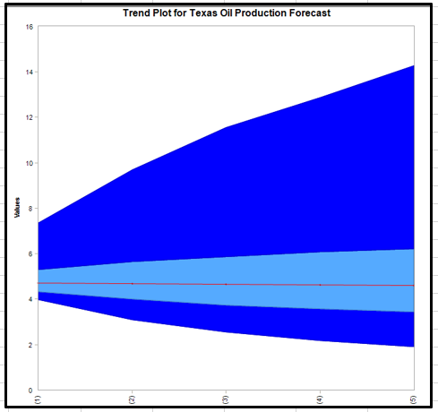
And now, we are ready to
forecast the next 5 years bellow:

The trend chart, suggest
that de median oil production is expected to be the same over the next 5 years.
One year into the future, the range of production is fairly narrow, but the
time a year passes, the forecast range extends from 2 mb/day to over an extreme
14 mb/day.
I will assume average value of distributions of oil production for each year as my base case:

Projection
of revenues for the next five years
In order to project
revenues into the future, I need to regress past revenues against a variable
that best fit my regression. Some candidates could be “WTI oil prices ($/barrel)”,
“gas oil prices” or “Texas oil production (mb/day)”, or a combination of these
variables.
I have tried several
combinations, but the best one is to focus on “Texas oil production”. Now you,
reader, can understand my effort in point 5 of this post.
If I run a regression
revenues against oil production (according our limited data from last 10 years),
we have an R-square high (75%) and an oil production coefficient highly
statistically significant (P-value = 0.001).
If I wish to forecast the
revenues that would result from whatever amount of oil production, we could use
the estimated relationship
Revenues ($ m) = -144.32 +
83.52 x Oil Production (mb/day)
But because of the limited
amount of data and because of chance, there is uncertainty about the true
relationship between oil production and revenues, and to simulate the
uncertainty in the relationship correctly, we need to adopt a different
procedure.
The method I will use is a
parametric Bootstrap. This procedure outputs bootstrap samples which are
constructed by simulating the sales level for each Oil Production level in the
original data set.
Finally, with my Bootstrap
model, I get Revenues for the next five years which are normal distributed as
follows:

In the figure above we observe
that the further we move away from the present, the wider our distributions and
less accurate our predictions, of course.
Again, I will assume average
value of distributions as my base case:


Final
Valuation
Now, we are ready to value
our company. In the next table I try to summarize my valuation

I was tempted to give some
probability to fail due to the next recession we face, but my probability is
zero because TPL has no competitor right now. My equity value is $2.439 billion,
there are 7.76 million shares outstanding, and my final valuation is $353.02 per
share.
The great deal of
uncertainty in this valuation are revenues for the next five years which are
driven by the oil production, but I can still estimate value in spite of that
uncertainty. In fact, that is what I have done in the simulation below:

In terms of base numbers,
the simulation does not change my view of TPL. My median value is $289.69, with
the tenth percentile at close to $147.81 and the ninetieth percentile at $576.11,
making it over valued, if it is priced at $457.00. The long tail on positive
end of the distribution implies that I would buy TPL with a smaller margin of
safety, because of the potential of significant upside.